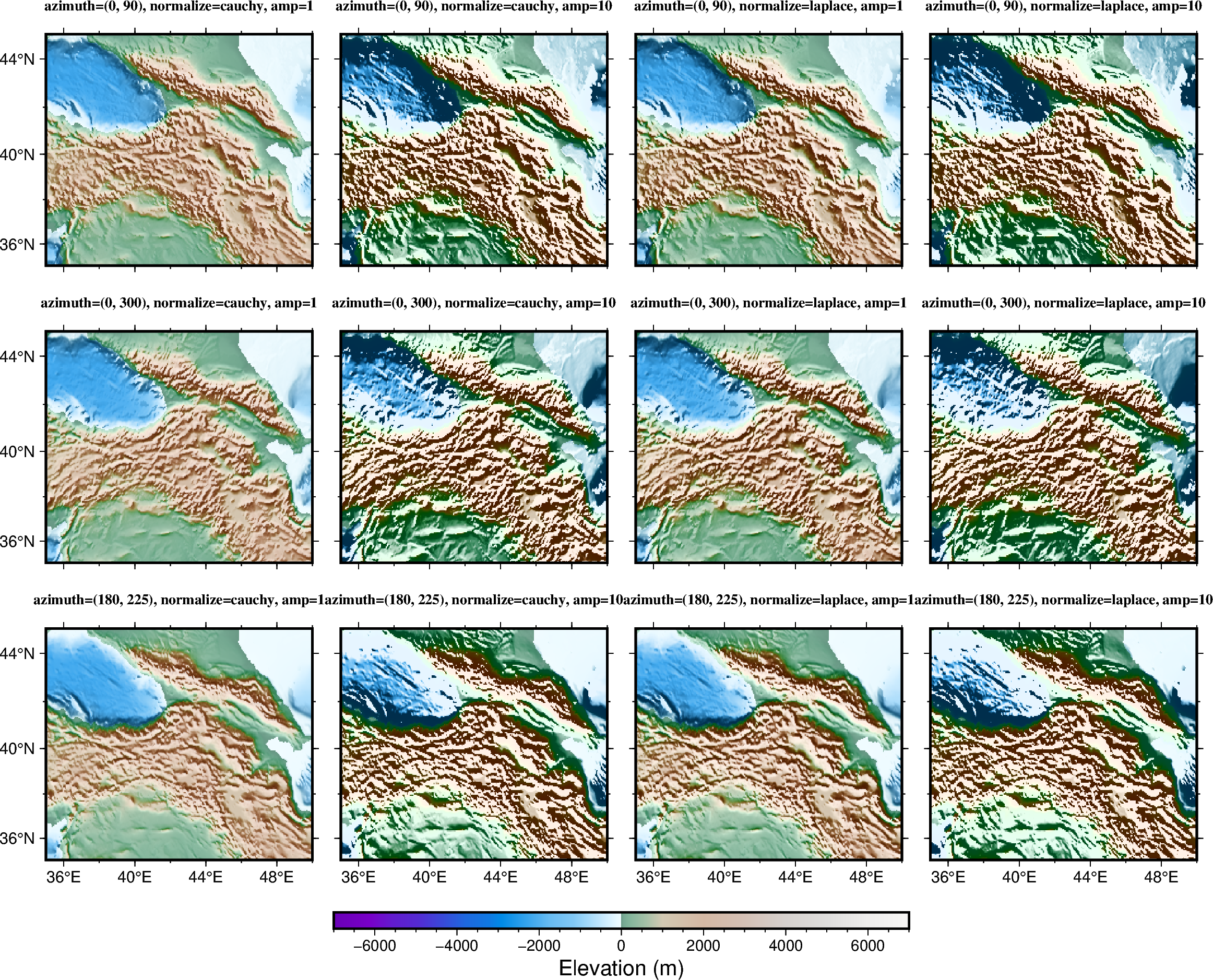
Calculating grid gradient with custom azimuth and normalization parameters

The pygmt.grdgradient function calculates the gradient of a grid file. As input, pygmt.grdgradient gets an xarray.DataArray object or a path string to a grid file. It then calculates the respective gradient and returns an xarray.DataArray object. The example below shows how to customize the gradient by setting azimuth and normalization parameters.

• azimuth sets the illumination light source direction (0° is North, 90° is East, 180° is South, 270° is West).

• normalize and related parameters enhances the 3-D sense of the topography.

The normalize parameter calculates the azimuthal gradient of each point along a certain azimuth angle, then adjusts the brightness value of the color according to the positive/negative of the azimuthal gradient and the amplitude of each point.

grdblend [NOTICE]: Remote data courtesy of GMT data server oceania [http://oceania.generic-mapping-tools.org]
grdblend [NOTICE]: SRTM15 Earth Relief v2.7 at 03x03 arc minutes reduced by Gaussian Cartesian filtering (15.7 km fullwidth) [Tozer et al., 2019].
grdblend [NOTICE]:   -> Download 90x90 degree grid tile (earth_relief_03m_g): N00E000

import pygmt
from pygmt.params import Position

# Load the 3 arc-minutes global relief grid in the target area around Caucasus
grid = pygmt.datasets.load_earth_relief(resolution="03m", region=[35, 50, 35, 45])

fig = pygmt.Figure()

# Define a colormap to be used for topography
pygmt.makecpt(cmap="gmt/terra", series=(-7000, 7000))

# Define figure configuration
pygmt.config(FONT_TITLE="10p,5", MAP_TITLE_OFFSET="1p", MAP_FRAME_TYPE="plain")

# Setup subplot panels with three rows and four columns
with fig.subplot(
    nrows=3,
    ncols=4,
    figsize=("28c", "21c"),
    sharex="b",
    sharey="l",
):
    # Setting azimuth angles, e.g. (0, 90) illuminates light source from the North (top)
    # and East (right).
    for azi in [(0, 90), (0, 300), (180, 225)]:
        # "cauchy"/"laplace" sets cumulative Cauchy/Laplace distribution, respectively.
        for normalize in ("cauchy", "laplace"):
            # amp (e.g., 1 or 10) controls the brightness value of the color.
            for amp in (1, 10):
                # Making an intensity DataArray using azimuth and normalize parameters
                shade = pygmt.grdgradient(
                    grid=grid, azimuth=azi, normalize=normalize, norm_amp=amp
                )
                fig.grdimage(
                    grid=grid,
                    shading=shade,
                    projection="M?",
                    frame=[
                        "a4f2",
                        f"+tazimuth={azi}, normalize={normalize}, amp={amp}",
                    ],
                    cmap=True,
                    panel=True,
                )

fig.colorbar(
    position=Position("BC", cstype="outside"),
    length=14,
    width=0.4,
    orientation="horizontal",
    frame="xa2000f500+lElevation (m)",
)

fig.show()